Getting started with joinery • joinery

The problem

You have two tables of people. They are the same people, typed by different hands on different days. One table writes Prof. Dr. Müller, the other writes Mueller. One has Bahnhofstraße 67a, the other Bahnhofstr. 67 A. First names collapse to initials. Middle names appear and disappear. Districts are spelled the same on both sides because nobody mistypes where they live.

An exact join finds none of these. Edit distance does a little better, but it trips on the things that matter: it counts Müller and Mueller as two edits apart, even though they are the same name, while rating genuinely different surnames that sit one letter apart, like Bauer and Mauer, as near. It has no idea that a rare surname is strong evidence and a common one is weak. It compares how strings look, when what you want to compare is the information two records share.

joinery takes the other route. It cuts each field into tokens, weights each token by how rare it is, and scores a pair by the rare tokens they have in common. This vignette walks the whole path on a pair of built-in tables, and then does something most linkage tutorials cannot: it scores the result against a known answer key.

How joinery thinks about a match

Take one real pair from the data we are about to load: a register row reading Amelie Hofmann, Konrad-Adenauer-Straße 2, Ronnenberg and a listing reading A. Hofmann, Konrad-Adenauer-Straße 2, Ronnenberg.

Tokens. Each field is cut into tokens, with the spelling smoothed first (lowercased, accents stripped) so that Amelie and amelie are the same token. The listing’s lone initial A. carries almost no information and will not match the register’s full amelie. How exactly each field is cut is the strategy you write in a moment.
Rarity. A token is worth more when it is rare. Hofmann is a common surname, so sharing it says something but not much. Ronnenberg is a rare place, so sharing it says a lot. This single idea is what separates joinery from edit-distance matching.
Overlap, not appearance. The two records are compared by the rare tokens they share, not by how their strings line up. The missing first name costs nothing, because the score is built from what the records have in common, not from what is absent.
Score and threshold. Each shared token contributes its share of its column’s weight. The contributions add up to a score between 0 and 1. A pair is kept when the score clears the threshold.
Entities. Records that link, directly or through a chain of links, form an entity: a duplicate group within one table, or a matched cluster across two.

The pair above scores exactly 0.80, and we will see later, token by token, exactly where that score came from. That per-token receipt is explain_match(), and it is the whole reason to prefer a transparent matcher: you can always ask why a pair scored what it did.

1. Look at the data

library(joinery)
library(dplyr)
#> 
#> Attaching package: 'dplyr'
#> The following objects are masked from 'package:stats':
#> 
#>     filter, lag
#> The following objects are masked from 'package:base':
#> 
#>     intersect, setdiff, setequal, union

data(base_example)
data(target_example)

glimpse(base_example)
#> Rows: 3,300
#> Columns: 7
#> $ id_base    <chr> "B0001", "B0002", "B0003", "B0004", "B0005", "B0006", "B000…
#> $ Vorname    <chr> "Hannah", "Hasan", "Peter", "Sophie", "Sarah", "Amelie", "T…
#> $ Nachname   <chr> "Wagner", "Demir", "Becker", "Lehmann", "Schmidt", "Hofmann…
#> $ Strasse    <chr> "Am Bahnhof", "Museumstraße", "Turmstraße", "Ringstraße", "…
#> $ Hausnummer <chr> "81", "20", "147", "38", "13", "2", "18", "141", "15", "20"…
#> $ Ort        <chr> "Laatzen", "Markkleeberg", "Sindelfingen", "Radebeul", "Köl…
#> $ Kreis      <chr> "Region Hannover", "Landkreis Leipzig", "Landkreis Böblinge…

joinery works directly with the data frames and tibbles you already have; there is nothing to convert. We use a few dplyr verbs below only to slice the results, not to feed joinery.

base_example is 3,300 person records. The last 300 are deliberate near-duplicates of earlier rows: the same people, re-entered with initials, added titles, dropped middle names, and house-number noise. That is the duplicate-detection case.

glimpse(target_example)
#> Rows: 3,000
#> Columns: 8
#> $ actual_link <chr> "B1763", "B2891", "B0743", "B0862", "B0625", "B2108", "B15…
#> $ Vorname     <chr> "Mustafa Ali", "Julia", "Daniel", "Marie", "K.", "Jürgen",…
#> $ Nachname    <chr> "Özkan", "Schröder", "Hoffmann", "Müllar", "Neumann", "Web…
#> $ Strasse     <chr> "Bahnhofstraße", "Wiener Straße", "Birkenweg", "Bahnhofstk…
#> $ Hausnummer  <chr> "67m", "79", "58", "73", "28", "70", "31", "1", "18B", "11…
#> $ Ort         <chr> "Offenbach", "Neusäß", "Neu-Isenburg", "Herzogenrath", "Bö…
#> $ Kreis       <chr> "Stadt Offenbach am Main", "Landkreis Augsburg", "Kreis Of…
#> $ id_target   <chr> "T1763", "T2891", "T0743", "T0862", "T0625", "T2108", "T15…

target_example is 3,000 records. About 80% are distorted copies of base_example people; the rest are genuinely new. The first column, actual_link, is the answer key: for every copied row it holds the true id_base it came from. That is unusual for a linkage tutorial and we will lean on it in section 7.

Inspect one known pair. Target row T0006 carries actual_link = "B0006":

target_example |>
  filter(id_target == "T0006") |>
  select(id_target, Vorname, Nachname, Strasse, Ort)
#> # A tibble: 1 × 5
#>   id_target Vorname Nachname Strasse                Ort       
#>   <chr>     <chr>   <chr>    <chr>                  <chr>     
#> 1 T0006     A.      Hofmann  Konrad-Adenauer-Straße Ronnenberg

base_example |>
  filter(id_base == "B0006") |>
  select(id_base, Vorname, Nachname, Strasse, Ort)
#> # A tibble: 1 × 5
#>   id_base Vorname Nachname Strasse                Ort       
#>   <chr>   <chr>   <chr>    <chr>                  <chr>     
#> 1 B0006   Amelie  Hofmann  Konrad-Adenauer-Straße Ronnenberg

Same person, Amelie shortened to A.. An exact join on name misses it.

Kreis (the administrative district) is the one field the noise leaves alone, so it makes a natural blocking key: only compare records that sit in the same district. That turns a 3,300 by 3,000 comparison into a handful of small ones.

2. Declare a strategy

Think of a strategy as a jig, a woodworker’s template that guides the same cut every time. You set it up once, then run it over every table. It says how to turn each column into tokens, how to block, and where to set the threshold. It runs nothing by itself.

strat <- search_strategy(
  Nachname   ~ normalize_text() + word_tokens(min_nchar = 3),
  Vorname    ~ normalize_text() + word_tokens(min_nchar = 3),
  Strasse    ~ normalize_street(lang = "de") + word_tokens(min_nchar = 3),
  Hausnummer ~ numeric_tokens,
  Ort        ~ normalize_text(),
  block_by   = "Kreis",
  threshold  = 0.8
)

strat
#> <joinery::Search_Strategy>
#> 
#> columns
#> Nachname: normalize_text() -> word_tokens(min_nchar = 3)
#> Vorname: normalize_text() -> word_tokens(min_nchar = 3)
#> Strasse: normalize_street(lang = "de") -> word_tokens(min_nchar = 3)
#> Hausnummer: numeric_tokens()
#> Ort: normalize_text()
#> 
#> blocking: Kreis
#> weights: none
#> rarity: inverse_freq (min=0)
#> fan-out guard: cap at 50,000,000
#> smoothing: none
#> threshold: 0.8
#> max_candidates: none
#> feedback_strength: none

Preparers: how a column becomes tokens

Each formula reads column ~ preparer1 + preparer2 + ...: a small pipeline, run left to right. The early steps smooth the text; the last step cuts it into tokens. The four preparers used above:

normalize_text() lowercases and strips accents, so casing and diacritics stop mattering.
normalize_street(lang = "de") expands German street abbreviations (str. becomes straße) before the text is cut.
word_tokens(min_nchar = 3) splits text into words and drops anything shorter than three characters, so a lone initial like A. falls out while Amelie stays.
numeric_tokens keeps only the digit runs. It takes no arguments, so it is written bare, without the ().

So Ort ~ normalize_text() smooths the town name but never splits it, keeping it as one token, while Nachname ~ normalize_text() + word_tokens(min_nchar = 3) smooths and splits. joinery ships many more preparers (phonetic encoders such as as_metaphone(), n-grams, stopword filters); the reference index lists them all.

The other arguments

The formulas are the only required part. The rest are tuning knobs with sensible defaults:

Argument	What it does	If you omit it
`block_by`	only compare records that share this column’s value	no blocking: every record is compared with every other (fine for small tables, costly for large ones)
`threshold`	the lowest score a pair can have and still be kept	defaults to `0.9`
`weights`	a named vector to make some columns count for more	every column counts equally
`rarity`	how a token’s rarity is measured	`"inverse_freq"`, where rarer tokens score higher
`max_candidates`	maximum candidate matches kept per record; only the top-scoring N are returned	no limit
`smoothing`	transforms rIP scores before aggregation, redistributing weight across rare and common tokens	identity (no transformation)
`feedback_strength`	penalises a pair when the rare tokens of one record only partially appear in the other	`0` (disabled)

Here block_by = "Kreis" restricts every comparison to within a district, and threshold = 0.8 loosens the default slightly. The three bottom rows in the table appear in the strategy print-out but are rarely needed: max_candidates, smoothing, and feedback_strength all default to “none” and can be left alone for most linkage tasks. There are further levers for large runs (min_rarity, max_token_df, and a fan-out guard); their defaults are safe, and ?search_strategy documents them. This strategy is the one block of new syntax in the package; the rest are verbs that consume it.

3. Will it work? (check before you match)

You do not have to run a match to find out whether a strategy is sound. Start by inspecting one column’s tokens:

head(inspect_tokens(base_example, "id_base", strat, Vorname), 8)
#> # A tibble: 8 × 3
#>   token  Vorname     n
#>   <chr>  <chr>   <int>
#> 1 HANNAH Hannah     71
#> 2 HASAN  Hasan      15
#> 3 PETER  Peter     132
#> 4 SOPHIE Sophie    128
#> 5 SARAH  Sarah      59
#> 6 AMELIE Amelie     61
#> 7 THOMAS Thomas     78
#> 8 LUKAS  Lukas      56

Then ask for a pre-match health check:

audit_strategy(base_example, "id_base", strat)
#> 
#> ── Strategy_Audit ──────────────────────────────────────────────────────────────
#> n_records: 3300
#> column token stats
#> Hausnummer: 3300 tokens, 217 unique (6.6%), na_rate=0.0%
#> Nachname: 3300 tokens, 50 unique (1.5%), na_rate=0.0%
#> Ort: 3300 tokens, 63 unique (1.9%), na_rate=0.0%
#> Strasse: 4134 tokens, 88 unique (2.1%), na_rate=0.0%
#> Vorname: 3229 tokens, 65 unique (2.0%), na_rate=0.0%
#> column rarity quantiles
#> Hausnummer: p50=0.5000, pct_low_rarity=0.0%
#> Nachname: p50=0.2500, pct_low_rarity=0.0%
#> Ort: p50=0.0200, pct_low_rarity=0.0%
#> Strasse: p50=0.3333, pct_low_rarity=0.0%
#> Vorname: p50=0.3333, pct_low_rarity=0.0%
#> blocks: 36 blocks, top1_share="16.3%"
#> est_comparisons: "309017"

audit_strategy() reports, per column, how many distinct tokens there are and how rare they run, plus the block layout and an estimate of how many comparisons the match will cost. Here the blocking cuts the work to about 309,000 comparisons instead of the ten million a full cross would need. If a column were all boilerplate (no rare tokens) or a block were so large it would make the comparison count unmanageable, this is where you would see it, before paying for the match.

When no blocking key is available, max_candidates offers a softer control: setting it to, say, 3 keeps only the three highest-scoring candidates per record, capping the output without changing which pairs are evaluated. It does not reduce computation the way blocking does, but it prevents a large result table when the threshold alone is too loose.

If a single hyper-common token (a frequent house number, say) were fanning a block out, rarity_distribution() would show it and let you set the min_rarity or max_token_df levers. We do not need it here.

4. Deduplicate the base table

Deduplication is just matching a table against itself with the same strategy.

dups <- detect_duplicates(base_example, id = "id_base", strategy = strat)

dups |>
  select(duplicate_group, id, score, rank) |>
  head()
#> # A tibble: 6 × 4
#>   duplicate_group id    score  rank
#>             <int> <chr> <dbl> <int>
#> 1               7 B0007   0.8     1
#> 2               7 B3066   0.8     2
#> 3              18 B0018   0.8     1
#> 4              18 B3149   0.8     2
#> 5              22 B0022   0.8     1
#> 6              22 B3187   0.8     2

deduplicate_table() collapses each duplicate group to a single record:

base_clean <- deduplicate_table(base_example, dups, id = "id_base")

nrow(base_example) - nrow(base_clean)
#> [1] 282

We planted exactly 300 duplicates (the last 300 rows), and the dedup recovers 282 of them. The rest are the 18 where the noise was heavy enough to drop the pair below 0.8, which is exactly the precision/recall trade-off we look at next.

5. Search across tables

Now link the cleaned base table to the target table:

matches <- search_candidates(
  base_clean,
  target_example,
  base_id   = "id_base",
  target_id = "id_target",
  strategy  = strat
)

matches |>
  select(match_id, score, source, id, Nachname, rank) |>
  head()
#> # A tibble: 6 × 6
#>   match_id score source id    Nachname  rank
#>      <int> <dbl> <chr>  <chr> <chr>    <int>
#> 1        1     1 base   B0003 Becker       1
#> 2        1     1 target T0003 Becker       2
#> 3        2     1 base   B0005 Schmidt      1
#> 4        2     1 target T0005 Schmidt      2
#> 5        3     1 base   B0010 Wagner       1
#> 6        3     1 target T0010 Wagner       2

Each match_id groups the two sides of one candidate pair: a base row and a target row. The score is the shared-rarity total; rank orders competing candidates for the same record.

6. Did it work, and why this pair?

Every match raises two questions: whether the result held together, and why a given pair scored what it did.

summarise_matches(matches, threshold = 0.8)
#> 
#> ── Match_Overview (candidates) ─────────────────────────────────────────────────
#> n_pairs_or_groups: "1803" n_records_involved: "3605"
#> coverage: base=NA target=NA
#> score summary
#> min: 0.800
#> q1: 0.800
#> median: 0.800
#> mean: 0.888
#> q3: 1.000
#> max: 1.000
#> candidates-per-record (top 5)
#> 1 candidate(s): 1801 record(s)
#> 2 candidate(s): 1 record(s)
#> ! median top-1 vs top-2 score gap is 0.000; matches are weakly decisive, consider raising threshold or `feedback_strength`.
#> ! 55.8% of pairs score within an epsilon of the decision threshold; consider `calibrate_matches()` to fit a post-retrieval false-positive filter.

The overview shows the score distribution and flags how many pairs sit close to the threshold. For why this pair, ask for the receipt. Take the Amelie/A. Hofmann pair from the start: find its match_id, then explain it.

mid <- matches |> filter(id == "T0006") |> pull(match_id) |> first()

receipt <- explain_match(
  matches, strat,
  base      = base_clean,
  id        = "id_base",
  target    = target_example,
  target_id = "id_target",
  match_id  = mid
)

receipt
#> <joinery::Match_Explanation> match 804
#> 
#> Records:
#> lhs id=B0006 source=base id_base=B0006 Vorname=Amelie Nachname=Hofmann
#> Strasse=Konrad-Adenauer-Straße Hausnummer=2 Ort=Ronnenberg Kreis=Region
#> Hannover actual_link=NA id_target=NA
#> rhs id=T0006 source=target id_base=NA Vorname=A.  Nachname=Hofmann
#> Strasse=Konrad-Adenauer-Straße Hausnummer=2 Ort=Ronnenberg Kreis=Region
#> Hannover actual_link=B0006 id_target=T0006
#> 
#> Score: 0.8000
#> 
#> Per-column contributions:
#> Hausnummer 0.2000 (1 shared token)
#> Nachname 0.2000 (1 shared token)
#> Ort 0.2000 (1 shared token)
#> Strasse 0.2000 (3 shared tokens)
#> 
#> Shared tokens (showing 6 of 6):
#> Hausnummer / 2 rarity=0.2500 rIP=1.0000 weight=0.2000 contrib=0.2000
#> Nachname / HOFMANN rarity=0.1250 rIP=1.0000 weight=0.2000 contrib=0.2000
#> Ort / RONNENBERG rarity=0.0114 rIP=1.0000 weight=0.2000 contrib=0.2000
#> Strasse / KONRAD rarity=0.0667 rIP=0.4648 weight=0.2000 contrib=0.0930
#> Strasse / ADENAUER rarity=0.0667 rIP=0.4648 weight=0.2000 contrib=0.0930
#> Strasse / STRASSE rarity=0.0101 rIP=0.0704 weight=0.2000 contrib=0.0141

This is the pair introduced in section 1. It scores exactly 0.80. The first name contributed nothing: the initial A. was shorter than the min_nchar = 3 cutoff and fell out of the token set. Nachname, Strasse, Hausnummer, and Ort each contributed 0.2, because the weights are equal and each of those columns returned at least one shared token.

The per-token receipt shows where the score came from and where it did not. Plotting it at token resolution makes the variation visible even when column totals are uniform:

token_contribution_plot(receipt)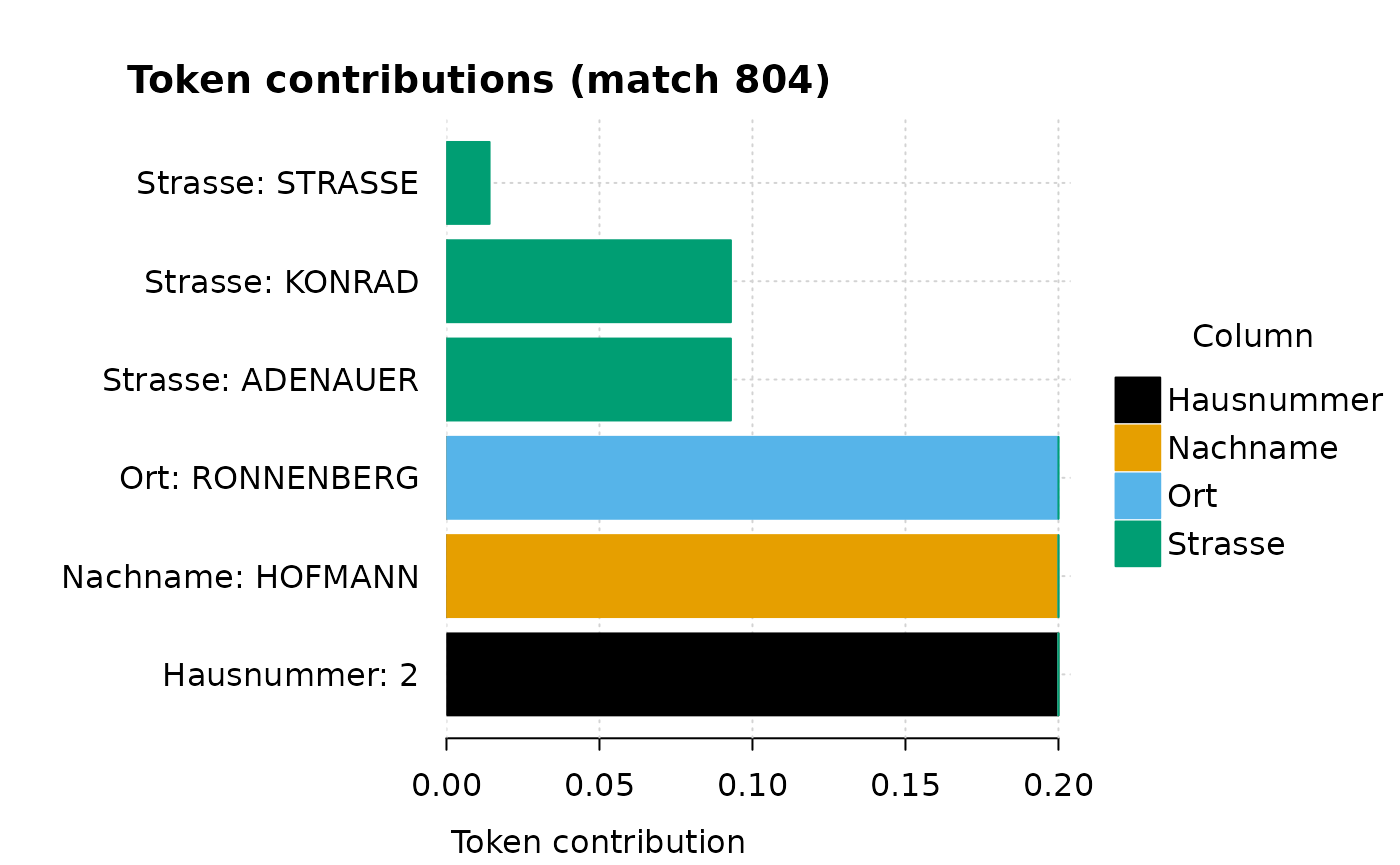

Horizontal bar chart of per-token contributions to the match score, coloured by column

Within Strasse, konrad and adenauer each contribute most of that column’s 0.2 share, while strasse (a word that appears on nearly every street) earns almost no rarity weight and contributes little despite being shared. Nothing about the score is hidden: every token shows its rarity, its rIP, and its contribution.

7. Score against the answer key

Because target_example$actual_link is ground truth, we can measure the match instead of trusting it. For each candidate pair, compare the base id we picked to the true link:

pred <- matches |>
  group_by(match_id) |>
  summarise(
    base_id = id[source == "base"][1],
    truth   = actual_link[source == "target"][1],
    .groups = "drop"
  ) |>
  mutate(correct = base_id == truth)

recoverable <- sum(target_example$actual_link %in% base_example$id_base)

c(
  pairs     = nrow(pred),
  precision = round(mean(pred$correct, na.rm = TRUE), 3),
  recall    = round(sum(pred$correct, na.rm = TRUE) / recoverable, 3)
)
#>     pairs precision    recall 
#>  1803.000     1.000     0.751

At threshold = 0.8 the matches are all correct (precision 1.0) and recover three quarters of the recoverable links (recall 0.75). The threshold is the dial between those two. The code below sweeps it across four values:

sweep <- bind_rows(lapply(c(0.6, 0.7, 0.8, 0.9), function(th) {
  st <- strat
  st@threshold <- th
  m <- search_candidates(base_clean, target_example,
                         base_id = "id_base", target_id = "id_target",
                         strategy = st)
  p <- m |>
    group_by(match_id) |>
    summarise(base_id = id[source == "base"][1],
              truth   = actual_link[source == "target"][1],
              .groups = "drop") |>
    mutate(correct = base_id == truth)
  tibble(
    threshold = th,
    pairs     = nrow(p),
    precision = round(mean(p$correct, na.rm = TRUE), 3),
    recall    = round(sum(p$correct, na.rm = TRUE) / recoverable, 3)
  )
}))

sweep
#> # A tibble: 4 × 4
#>   threshold pairs precision recall
#>       <dbl> <int>     <dbl>  <dbl>
#> 1       0.6  2484     0.942  0.95 
#> 2       0.7  1814     1      0.755
#> 3       0.8  1803     1      0.751
#> 4       0.9   792     1      0.33

Dropping to 0.6 lifts recall from 0.75 to 0.95, at the cost of a few false links (precision 0.94). Raising to 0.9 keeps precision perfect but throws away two thirds of the true matches. There is no single right answer; the right threshold depends on whether a missed link or a wrong link costs you more. When you need to do better than a single dial, a trained false-positive filter (calibrate_matches()) learns the boundary from labelled pairs.

8. Multistage matching

One pass rarely catches everything. The records a match did not touch are its residual:

unmatched_base   <- extract_unmatched(base_clean, "id_base", matches)
unmatched_target <- extract_unmatched(target_example, "id_target", matches)

nrow(unmatched_base)
#> [1] 1216
nrow(unmatched_target)
#> [1] 1197

multi_stage_search() handles these residuals automatically; you do not need to extract and pass them yourself. The calls below show how.

Exact matching as a first gate

The standard approach is to layer passes: a cheap exact stage first, then a tolerant fuzzy stage only on what is left. The layering logic is that the exact stage clears the easy cases (pairs where one record’s token set is fully contained in the other’s) before the heavier scoring starts on the harder residual.

An exact_strategy() matches pairs where one record’s token set for each column is fully contained in the other’s. The score is always 1.0; there is no rarity weighting and no threshold to tune. It is fast and produces zero false positives, so it is a reliable first gate. It takes the same column formulas as a search_strategy(), but weights, min_rarity, and thresholds are ignored: the match criterion is binary containment.

Composing stages

multi_stage_search() composes the stages in one call: it runs the exact strategy, extracts the residual, runs the fuzzy strategy on what is left, and merges the results into a single entity ledger.

staged <- multi_stage_search(
  base_clean, target_example,
  base_id   = "id_base",
  target_id = "id_target",
  strategies = list(
    exact = exact_strategy(
      Nachname ~ normalize_text() + word_tokens(min_nchar = 3),
      Vorname  ~ normalize_text() + word_tokens(min_nchar = 3),
      Ort      ~ normalize_text(),
      block_by = "Kreis"
    ),
    fuzzy = strat
  )
)

table(staged$stage)
#> 
#> exact fuzzy 
#>  2227  1486

The stage labels come from the names given in the strategies list — here "exact" and "fuzzy" — showing how many records each pass placed. Each row in the result ties a record to the entity it landed in and is tagged with the stage that placed it. Records claimed by the exact stage never enter the fuzzy stage, so the fuzzy scorer works on a smaller and harder problem. You can add as many stages as needed, each with a progressively looser strategy operating on the residual of the previous, and the ledger tracks which stage placed each record.

For deduplicating a single table the same way, use multi_stage_dedup(); it runs the same staged logic and resolves connected components at the end.

9. Where to look next

You now have the spine: declare a strategy, check it, dedup, search, score, stage. Four articles take it further, each framed around one problem:

Beyond the basics: fuzzy and exact strategies walks the advanced joins (containment, region-free movers, phonetic encoders, the fan-out guard) on the workshop_register / workshop_listings tables, where each feature has a planted case that measurably wins when you switch it on.
Matching across years and sources pools a multi-year panel and follows each workshop through time with a staged self-search.
Calibrating a false-positive filter trains a model on labelled pairs (sample_matches(), export_for_labelling(), fit_filter(), calibrate_matches()) for when one threshold is not enough.
Embedding-based matching matches on meaning instead of spelling, for records that share no tokens at all.

And two more pointers for planning and scale: plan_strategy() helps choose a blocking key on a dataset you do not know yet, and the same verbs run on a DuckDB connection when the data is too large for memory.